Using R to remove the outliers(Tukey’s IQR)/Rを用いて外れ値の除去(Tukey’s IQR法)

English

During experiments, data collection often results in outliers due to various factors such as experimental errors and individual differences among subjects. These outliers are unavoidable and can be a major source of inaccuracy in data analysis. Proper removing of outliers is crucial to achieving reliable experimental results, especially in data modeling (e.g., regression analysis), where appropriately managing outliers is a critical step before model building.

What is an Outlier?

An outlier is a data point that deviates significantly from the expected range based on logical or empirical standards. For example, in a dataset where most values fall between 100 and 120, a value of 200 would clearly be an outlier. While small deviations may not significantly impact results in smaller samples, a value of 1000 would necessitate attention as it could severely distort the data analysis. Therefore, the accurate identification and management of outliers are essential.

Identifying Outliers

During my master’s and doctoral research, I conducted most experiments in a controlled lab environment, allowing me to manually identify and exclude outliers based on experience. This process required extensive practice to refine the skill of discerning outliers accurately. For example, selecting representative subjects for measurement and strategically excluding indirectly derived data points are decisions that heavily rely on accumulated experience.

Currently, my work involves removing much larger datasets from field trials and large-scale greenhouse studies, where the volume of data far exceeds what I dealt with previously. This shift has introduced the challenge of rapidly and accurately removing outliers, especially given my limited familiarity with the growth patterns of certain crops. Additionally, field experiments are typically conducted only once per year, slowing the accumulation of experience and complicating subsequent data analyses.

Addressing outliers effectively requires practical experience, as these values can often hold critical insights. Therefore, judgments about outliers should be grounded in a realistic understanding of the data, avoiding rash decisions that could lead to significant errors. For large datasets, boxplots are commonly used in academic research to visually represent the distribution and potential outliers within the data.

Removing Outliers

As previously mentioned, outliers can significantly affect data analysis because many statistical metrics, such as mean, standard deviation, and correlation, are highly sensitive to them. Any statistical calculation based on these metrics is vulnerable to distortion by outliers. Whether removing outliers is beneficial depends on their impact on the model—positive or negative. It is important to remember that outliers do not always indicate incorrect observations or flawed experiments; they may also represent natural variations or significant discoveries within the data. Therefore, deciding whether to remove or retain an outlier requires careful consideration, and data points should not be discarded merely because they seem unusual.

Typically, manual identification of outliers focuses on extreme values. According to the principles of normal distribution, isolated extreme values can often be removed without significantly affecting the overall distribution or validity of the data. However, when extreme values are clustered, this method becomes inadequate.

To address this, statisticians have developed several methods for detecting outliers, with the Z-score and Interquartile Range (IQR) methods being among the most commonly used. Below, I introduce a custom function based on Tukey’s IQR method, which effectively identifies outliers while minimizing the influence of extreme values on the mean and standard deviation, ensuring more robust analysis results.

Code in R

Define a function to remove outliers and generate comparative plots of the data with and without outliers.

#Define a function
outlierKD <- function(dt, var) {
var_name <- eval(substitute(var),eval(dt))
tot <- sum(!is.na(var_name))
na1 <- sum(is.na(var_name))
m1 <- mean(var_name, na.rm = T)
par(mfrow=c(2, 2), oma=c(0,0,3,0))
boxplot(var_name, main="With outliers")
hist(var_name, main="With outliers", xlab=NA, ylab=NA)
outlier <- boxplot.stats(var_name)$out
mo <- mean(outlier)
var_name <- ifelse(var_name %in% outlier, NA, var_name)
boxplot(var_name, main="Without outliers")
hist(var_name, main="Without outliers", xlab=NA, ylab=NA)
title("Outlier Check", outer=TRUE)
na2 <- sum(is.na(var_name))
cat("Outliers identified:", na2 - na1, "\n")
cat("Propotion (%) of outliers:", round((na2 - na1) / tot*100, 1), "\n")
cat("Mean of the outliers:", round(mo, 2), "\n")
m2 <- mean(var_name, na.rm = T)
cat("Mean without removing outliers:", round(m1, 2), "\n")
cat("Mean if we remove outliers:", round(m2, 2), "\n")
response <- readline(prompt="Do you want to remove outliers and to replace with NA? [yes/no]: ")
if(response == "y" | response == "yes"){
dt[as.character(substitute(var))] <- invisible(var_name)
assign(as.character(as.list(match.call())$dt), dt, envir = .GlobalEnv)
cat("Outliers successfully removed", "\n")
return(invisible(dt))
} else{
cat("Nothing changed", "\n")
return(invisible(var_name))
}
}

The custom function has only two parameters: the first is the dataset name, and the second is the variable name. By correctly substituting the dataset and variable name, the code can be executed directly. In this function, we define outliers based on the boxplot criteria, but this can be adjusted based on expert knowledge, such as defining outliers as values greater than or less than mean ± 3 SD. At the end of the function, user input will be prompted, allowing users to decide whether to remove the identified outliers by typing “yes” or “no.”

Here, I demonstrate the function using my own greenhouse crop fresh weight data to validate its performance.

Read csv data and make a dataframe (df) for analysis.

#read data
> data <- read.csv("125.csv", header = TRUE)
> df_list <- list()
> first<- data[,2] #There are 18 columns in my dataframe, I choose the second as example
> df <- data.frame(bp = first)

Run the “OutlierKD”

#read data
#run function for removing outliers
> outlierKD(df, bp)
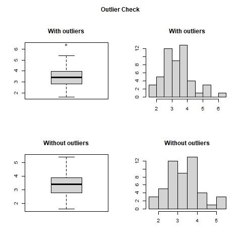
Outliers identified: 1 
Propotion (%) of outliers: 2 
Mean of the outliers: 6.4 
Mean without removing outliers: 3.43 
Mean if we remove outliers: 3.37 
Do you want to remove outliers and to replace with NA? [yes/no]: yes 
Outliers successfully removed 

After running the outlierKD function, a prompt appears with a “yes/no” option. Based on the described mean values and the generated boxplot or histogram, we can decide whether to remove the outliers. In this case, we found that the difference between the data before and after outlier removal was only 0.06, with an outlier ratio of 2%. Therefore, we chose “yes.”

As a result, we obtained a new dataframe (df). Let’s compare the differences between the original and the modified dataframes.

#combine two "df" in a df_list
df_list1 <- list(first,df2)
> names(df_list1) <- c("with outliers","without outliers")
> df_list
$`with outliers`
 [1] 4.0 2.9 3.0 4.5 3.5 3.8 4.1 4.3 3.9 2.6 3.3  NA 2.8 3.4  NA  NA 5.4 5.1 3.7
[20] 3.4 2.8 1.7 6.4 3.1 2.6 3.4 3.9  NA 3.6 2.6 2.7 2.9 2.1 4.0 2.5 1.6 3.0 4.0
[39] 2.4  NA 1.9 2.5 3.6 3.4 3.0 3.4 3.0 5.3 3.4 3.6 2.4 4.2 3.9 3.6  NA  NA 4.8
[58] 4.0  NA  NA

$`without outliers`
 [1] 4.0 2.9 3.0 4.5 3.5 3.8 4.1 4.3 3.9 2.6 3.3  NA 2.8 3.4  NA  NA 5.4 5.1 3.7
[20] 3.4 2.8 1.7  NA 3.1 2.6 3.4 3.9  NA 3.6 2.6 2.7 2.9 2.1 4.0 2.5 1.6 3.0 4.0
[39] 2.4  NA 1.9 2.5 3.6 3.4 3.0 3.4 3.0 5.3 3.4 3.6 2.4 4.2 3.9 3.6  NA  NA 4.8
[58] 4.0  NA  NA

Based on the plots and the data discussed above, we can see that the function successfully removed the outlier “6.4,” and its removal had minimal impact on the overall mean of the dataset.

Using just two simple commands, I was able to eliminate the outliers from the dataset, demonstrating one of the most efficient methods available. R offers many other techniques for removing outliers, which are commonly used in data processing. However, quickly removing outliers without proper investigation is not considered good statistical practice. Outliers are inherently part of the dataset and may carry important information, and their removal could lead to model inconsistencies.

Additionally, I will provide an example of batch outlier removal using my greenhouse data, which consists of an 18 × 60 dataset (18 varieties, n = 60, including NA values).

outlierKD <- function(dt, var, index) {
  var_name <- eval(substitute(var), eval(dt))
  tot <- sum(!is.na(var_name))
  na1 <- sum(is.na(var_name))
  m1 <- mean(var_name, na.rm = TRUE)
  par(mfrow = c(2, 2), oma = c(0, 0, 3, 0))
  boxplot(var_name, main = "With outliers")
  hist(var_name,
       main = "With outliers",
       xlab = NA,
       ylab = NA)
  outlier <- boxplot.stats(var_name)$out
  mo <- mean(outlier)
  var_name <- ifelse(var_name %in% outlier, NA, var_name)
  boxplot(var_name, main = "Without outliers")
  hist(var_name,
       main = "Without outliers",
       xlab = NA,
       ylab = NA)
  title("Outlier Check", outer = TRUE)
  na2 <- sum(is.na(var_name))
  cat("Outliers identified:", na2 - na1, "\n")
  cat("Propotion (%) of outliers:", round((na2 - na1) / tot * 100, 1), "\n")
  cat("Mean of the outliers:", round(mo, 2), "\n")
  m2 <- mean(var_name, na.rm = TRUE)
  cat("Mean without removing outliers:", round(m1, 2), "\n")
  cat("Mean if we remove outliers:", round(m2, 2), "\n")
  response <- "yes"  # 将默认回答设为 "yes"
  if (response == "y" | response == "yes") {
    dt[as.character(substitute(var))] <- invisible(var_name)
    assign(as.character(as.list(match.call())$dt), dt, envir = .GlobalEnv)
    cat("Outliers successfully removed", "\n")
    return(invisible(dt))
  } else{
    cat("Nothing changed", "\n")
    return(invisible(var_name))
  }
}

Here, I modified the default code to automatically remove all outliers by setting the default response to “yes.” The 18 × 60 CSV file is read, where each column represents the data for a specific variety. Therefore, when removing outliers, each column must be evaluated separately rather than treating all 1,080 data points collectively for outlier removal.

# Read CSV file
#data <- read.csv("125.csv", header = TRUE)

# Creat a new dataframe for collection of new data
df_list <- list()

The data was processed in batches, divided into 18 iterations. In each iteration, the data with outliers removed was saved and written into a list of dataframes.(df_list).

# Loop through each column of data; each column is compared independently. This example has 18 columns, indexed from 1 to 18.
for (i in 1:18) {
  # Extract the i-th column of data
  first <- data[, i]
  
  # Place the first column of data into a dataframe
  df <- data.frame(bp = first)
  
  # Call the outlier detection and handling function and save the generated plot
  jpeg(paste0("plot_", i, ".jpg"))
  outlierKD(df, bp, i)
  dev.off()
  
  # Save the processed dataframe
  df_list[[i]] <- df$bp
}

# Merge the data from the 18 iterations and save it as a new CSV file
# Combine the processed dataframes
combined_df <- data.frame(df_list)

# Naming the columns; here, I default to naming them as varieties 1-18, but you can adjust as needed
names(combined_df) <- c(1:18)

# Save the combined dataframe to a CSV file
write.csv(combined_df, file = "combined_data.csv", row.names = FALSE)

These procedures pertain to the handling of my greenhouse data. I also manage numerous field experiments, where each location can contain tens of thousands of data points. Applying such methods could significantly reduce the workload. Nonetheless, the decision to remove outliers should be made with careful consideration by both the experimental designer and the practitioner.

日本語

実験中にデータ収集を行うと、実験誤差や被験者間の個体差など、さまざまな要因によって外れ値が生じることがよくある。これらの外れ値は避けられないものであり、データ分析において重要な不正確さの原因となる。外れ値を適切に除去することは、信頼性のある実験結果を得るために重要であり、特にデータモデリング（例えば回帰分析）では、モデル構築前に外れ値を適切に分析することが重要なステップとなる。

外れ値とは何か？

外れ値とは、論理的または経験的基準に基づいて予期される範囲から大きく逸脱したデータポイントである。例えば、データセット内のほとんどの値が100から120の範囲にある場合、200という値は明らかに外れ値である。小さな逸脱はサンプルサイズが小さい場合には結果に大きな影響を与えないこともあるが、1000という値は注意が必要であり、データ分析を著しく歪める可能性がある。したがって、外れ値の正確な判定と対処は不可欠である。

外れ値の判定

私の修士・博士課程の研究では、ほとんどの実験は実験室で行い、経験に基づいて外れ値を手動で特定し除去していた。このプロセスには、外れ値を正確に見分けるスキルを磨くための広範な実践が必要であった。例えば、測定のために代表的な対象を選定し、間接的に得られたデータポイントを除外する決定は、蓄積された経験に大きく依存している。

現在、私の作業はフィールド試験や大規模な温室研究から得られるはるかに大規模なデータセットを扱っており、データ量は以前のものを大きく上回る。この変化により、特に特定の作物の成長パターンに対する知識が限られているため、外れ値を迅速かつ正確に除去するという問題が生じている。さらに、フィールド実験は通常年に一度しか行われず、経験の蓄積が遅く、データの分析がさらに複雑になる。

外れ値に効果的に対処するためには実践的な経験が必要であり、これらの値はしばしば重要な洞察を含んでいる可能性がある。したがって、外れ値についての判断はデータの現実的な理解に基づくべきであり、大きなエラーを引き起こす可能性のある軽率な決定を避けるべきである。大規模なデータセットに対しては、ボックスプロットがデータの分布と潜在的な外れ値を視覚的に表現するために広く使用されている。

外れ値の除去

前述のように、外れ値はデータ分析に大きな影響を与える可能性があり、多くの統計指標（例えば平均、標準偏差、相関）は外れ値に対して非常に敏感である。これらの指標に基づく統計計算は、外れ値によって歪められる可能性がある。外れ値を除去することが有益かどうかは、モデルへの影響—ポジティブかネガティブか—によって異なる。外れ値は常に不正確な観測結果や欠陥のある実験を示すものではなく、データ内の自然な変動や重要な発見を示している可能性があることを忘れてはならない。したがって、外れ値を除去するか保持するかの決定は慎重に行うべきであり、単に異常に見えるからといってデータポイントを捨てるべきではない。

通常、外れ値の手動識別は極端な値に焦点を当てる。正規分布の原則によれば、孤立した極端な値は全体の分布やデータの有効性に大きな影響を与えることなく除去できる。しかし、極端な値がクラスターを形成している場合、この方法は不十分になる。

この問題に対処するために、統計学者は外れ値を検出するためのいくつかの方法を開発しており、Zスコア法や四分位範囲（IQR）法が最も一般的に使用される方法の一部である。以下に、TukeyのIQR法に基づくカスタム関数を紹介し、極端な値が平均や標準偏差に与える影響を最小限に抑えながら外れ値を効果的に特定する方法を示す。

Rコード

外れ値を除去し、外れ値の有無でデータを比較するプロットを生成する関数を定義する。

#関数を定義する
outlierKD <- function(dt, var) {
var_name <- eval(substitute(var),eval(dt))
tot <- sum(!is.na(var_name))
na1 <- sum(is.na(var_name))
m1 <- mean(var_name, na.rm = T)
par(mfrow=c(2, 2), oma=c(0,0,3,0))
boxplot(var_name, main="With outliers")
hist(var_name, main="With outliers", xlab=NA, ylab=NA)
outlier <- boxplot.stats(var_name)$out
mo <- mean(outlier)
var_name <- ifelse(var_name %in% outlier, NA, var_name)
boxplot(var_name, main="Without outliers")
hist(var_name, main="Without outliers", xlab=NA, ylab=NA)
title("Outlier Check", outer=TRUE)
na2 <- sum(is.na(var_name))
cat("Outliers identified:", na2 - na1, "\n")
cat("Propotion (%) of outliers:", round((na2 - na1) / tot*100, 1), "\n")
cat("Mean of the outliers:", round(mo, 2), "\n")
m2 <- mean(var_name, na.rm = T)
cat("Mean without removing outliers:", round(m1, 2), "\n")
cat("Mean if we remove outliers:", round(m2, 2), "\n")
response <- readline(prompt="Do you want to remove outliers and to replace with NA? [yes/no]: ")
if(response == "y" | response == "yes"){
dt[as.character(substitute(var))] <- invisible(var_name)
assign(as.character(as.list(match.call())$dt), dt, envir = .GlobalEnv)
cat("Outliers successfully removed", "\n")
return(invisible(dt))
} else{
cat("Nothing changed", "\n")
return(invisible(var_name))
}
}

カスタム関数には2つのパラメータがある。最初のパラメータはデータセット名、2つ目のパラメータは変数名である。データセット名と変数名を正しく置き換えることで、コードを直接実行することができる。この関数では、ボックスプロットの基準に基づいて外れ値を定義しているが、専門的な知識に基づいて、例えば平均 ± 3 標準偏差の値を外れ値と定義するなど、調整が可能である。関数の最後でユーザーに入力を促し、識別された外れ値を除去するかどうかを “yes” または “no” と入力して決定することができる。

ここでは、自分の温室作物の生鮮重データを用いて、関数の性能を検証する。

CSVデータを読み込み、分析のためのデータフレーム（df）を作成する。

#read data
> data <- read.csv("125.csv", header = TRUE)
> df_list <- list()
> first<- data[,2] #There are 18 columns in my dataframe, I choose the second as example
> df <- data.frame(bp = first)

「OutlierKD」を実行する

#read data
#run function for removing outliers
> outlierKD(df, bp)
Outliers identified: 1 
Propotion (%) of outliers: 2 
Mean of the outliers: 6.4 
Mean without removing outliers: 3.43 
Mean if we remove outliers: 3.37 
Do you want to remove outliers and to replace with NA? [yes/no]: yes 
Outliers successfully removed 

outlierKD 関数を実行すると、「yes/no」の選択肢が表示される。説明された平均値や生成されたボックスプロットやヒストグラムに基づいて、外れ値を除去するかどうかを決定する。この場合、外れ値除去前後のデータの差はわずか0.06で、外れ値の割合は2%だった。したがって、「yes」を選択した。

その結果、新しいデータフレーム（df）を得た。元のデータフレームと修正後のデータフレームの違いを比較する。

#2つの「df」を「df_list」に結合する
df_list1 <- list(first,df2)
> names(df_list1) <- c("with outliers","without outliers")
> df_list
$`with outliers`
 [1] 4.0 2.9 3.0 4.5 3.5 3.8 4.1 4.3 3.9 2.6 3.3  NA 2.8 3.4  NA  NA 5.4 5.1 3.7
[20] 3.4 2.8 1.7 6.4 3.1 2.6 3.4 3.9  NA 3.6 2.6 2.7 2.9 2.1 4.0 2.5 1.6 3.0 4.0
[39] 2.4  NA 1.9 2.5 3.6 3.4 3.0 3.4 3.0 5.3 3.4 3.6 2.4 4.2 3.9 3.6  NA  NA 4.8
[58] 4.0  NA  NA

$`without outliers`
 [1] 4.0 2.9 3.0 4.5 3.5 3.8 4.1 4.3 3.9 2.6 3.3  NA 2.8 3.4  NA  NA 5.4 5.1 3.7
[20] 3.4 2.8 1.7  NA 3.1 2.6 3.4 3.9  NA 3.6 2.6 2.7 2.9 2.1 4.0 2.5 1.6 3.0 4.0
[39] 2.4  NA 1.9 2.5 3.6 3.4 3.0 3.4 3.0 5.3 3.4 3.6 2.4 4.2 3.9 3.6  NA  NA 4.8
[58] 4.0  NA  NA

上記のプロットとデータに基づいて、関数が外れ値「6.4」を正しく除去し、その除去がデータセット全体の平均にほとんど影響を与えなかったことがわかる。

2つの簡単なコマンドを使って、データセットから外れ値を除去することができ、これは利用可能な最も効率的な方法の一つを示している。Rには外れ値を除去するための多くの他の技術があり、これらはデータ処理で一般的に使用される。しかし、適切な調査なしに外れ値を迅速に除去することは良い統計的手法とは言えない。外れ値は本質的にデータセットの一部であり、重要な情報を含んでいる可能性があり、その除去がモデルの不一致を引き起こす可能性がある。

さらに、私の温室データを使用したバッチ外れ値除去の例を示す。このデータは18 × 60のデータセット（18品種、n = 60、NA値を含む）で構成されている。

outlierKD <- function(dt, var, index) {
  var_name <- eval(substitute(var), eval(dt))
  tot <- sum(!is.na(var_name))
  na1 <- sum(is.na(var_name))
  m1 <- mean(var_name, na.rm = TRUE)
  par(mfrow = c(2, 2), oma = c(0, 0, 3, 0))
  boxplot(var_name, main = "With outliers")
  hist(var_name,
       main = "With outliers",
       xlab = NA,
       ylab = NA)
  outlier <- boxplot.stats(var_name)$out
  mo <- mean(outlier)
  var_name <- ifelse(var_name %in% outlier, NA, var_name)
  boxplot(var_name, main = "Without outliers")
  hist(var_name,
       main = "Without outliers",
       xlab = NA,
       ylab = NA)
  title("Outlier Check", outer = TRUE)
  na2 <- sum(is.na(var_name))
  cat("Outliers identified:", na2 - na1, "\n")
  cat("Propotion (%) of outliers:", round((na2 - na1) / tot * 100, 1), "\n")
  cat("Mean of the outliers:", round(mo, 2), "\n")
  m2 <- mean(var_name, na.rm = TRUE)
  cat("Mean without removing outliers:", round(m1, 2), "\n")
  cat("Mean if we remove outliers:", round(m2, 2), "\n")
  response <- "yes"  # 将默认回答设为 "yes"
  if (response == "y" | response == "yes") {
    dt[as.character(substitute(var))] <- invisible(var_name)
    assign(as.character(as.list(match.call())$dt), dt, envir = .GlobalEnv)
    cat("Outliers successfully removed", "\n")
    return(invisible(dt))
  } else{
    cat("Nothing changed", "\n")
    return(invisible(var_name))
  }
}

ここでは、デフォルトコードを修正して、デフォルトの応答を「yes」に設定し、すべての外れ値を自動的に除去するようにした。18 × 60のCSVファイルを読み込み、各列が特定の品種のデータを表している。そのため、外れ値を除去する際は、全ての1,080データポイントを一括で扱うのではなく、各列をそれぞれに評価する必要がある。

# csvファイル読む
#data <- read.csv("125.csv", header = TRUE)

# Creat a new dataframe for collection of new data
df_list <- list()

データはバッチ処理され、18回のイテレーションに分けられた。各イテレーションで、外れ値が除去されたデータが保存され、データフレームのリストに書き込まれた。

# 各列のデータをループ処理する; 各列は独立して比較される。この例では18列があり、1から18までインデックス付けされている。
for (i in 1:18) {
  # i番目の列のデータを抽出する
  first <- data[, i]
  
  # 抽出した列のデータをデータフレームに格納する
  df <- data.frame(bp = first)
  
  # 外れ値検出および処理関数を呼び出し、生成されたプロットを保存する
  jpeg(paste0("plot_", i, ".jpg"))
  outlierKD(df, bp, i)
  dev.off()
  
  # 処理されたデータフレームを保存する
  df_list[[i]] <- df$bp
}

# 18回のループから得られたデータを統合し、新しいCSVファイルとして保存する
# 処理されたデータフレームを結合する
combined_df <- data.frame(df_list)

# 列に名前を付ける; ここでは品種1-18とデフォルトで名付けているが、必要に応じて調整可能
names(combined_df) <- c(1:18)

# 統合されたデータフレームをCSVファイルとして保存する
write.csv(combined_df, file = "combined_data.csv", row.names = FALSE)

最後、これらの手順は私の温室データの処理に関連している。さらに、多くの大田実験も管理しており、各ロケーションには数万のデータポイントが含まれることがある。このような方法を適用することで、作業負荷を大幅に削減できる。しかし、外れ値を除去する決定は、実験デザイナーと実施者の両方が慎重に考慮する必要がある。